Free Trade Equilibrium Graph
Small Country Case where PFT is the free trade equilibrium price. Small Country Case The free trade price P FT is the price that prevails in the export or world market.
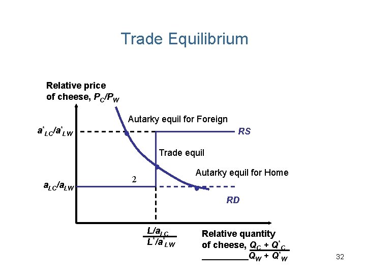
Autarky Equilibrium
What is the volume of trade.
Free trade equilibrium graph. See Figure 75 Depicting a Free Trade Equilibrium. See Figure 75 Depicting a Free Trade Equilibrium. These equilibrium points are labeled with the point E.
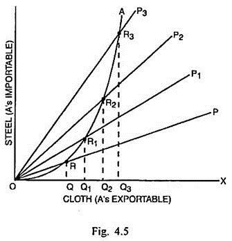
Notice that in this set-up Brazil is the low-cost provider of sugar and has the cost-advantage. Consider the following data on the factor endowments of two countries A and B. Show the free trade equilibrium of the country in a diagram placing clothing on horizontal axis and food on the vertical axis.
Graph the equilibrium under free trade. The supply and demand curves for the two countries are shown in the adjoining diagram. Export supply with Mexican import demand.
Algebraically the free trade price is the. What is the world price. Preferred and Affordable Sets.
Export supply with Mexican import demand determines the equilibrium free trade price P FT and the quantity traded Q FT where Q FT XS US P FT MD Mex P FT. Thats the horizontal distance between the supply and demand curves at the free. K 60 machines 10 machines Continue reading Free trade equilibrium on each graph.
The Sugar Trade between Brazil and the United. Perfect Complements Utility 3D Perfect Substitites Utility 3D Quasilinear Utility 3D Concave Utility 3D MRS and Marginal Utility 3D MRS Along an Indifference Curve 3D Constrained Optimization. Utility Maximization Subject to a Budget Constraint.
Consider the following data on the factor endowments of two countries A and B. The supply curve represents the quantity of wheat that US producers would be willing to supply at every potential price for wheat in the US market. Please use one graph per country and show both the autarkyand the free trade equilibrium on each graph.
Get Your Custom Essay on Free trade equilibrium on each graph Just from 13Page Order Essay Countries Factor Endowments A. Consider the following data on the factor endowments of two countries A and B. Describe the patterns of specialisation and trade.
Draw the graph carefully. Please use one graph per country and show both the autarkyand the free trade equilibrium on each graph. Countries Factor Endowments A B Labor force.
The free trade equilibrium is depicted in Figure 718 Welfare Effects of a Tariff. The free trade productionconsumption bundle would not have been a choice given autarky prices Figure 3 illustrate that at trade prices the domestic consumption bundle is. The quantity of imports and exports is shown as the blue line segment on each countrys graph.
The free trade price P FT must be the price that equalizes the US. Export supply with Mexican import demand. In this case the free-trade equilibrium black plus occurs at a price of 400 per barrel of oil and a.
When there is no trade in the United States the equilibrium price of sugar is 24 cents per pound and the equilibrium quantity is 80 tons. Please use one graph per country and show both the autarkyand the free trade equilibrium on each graph. At that price domestic demand is given by DFT domestic supply by SFT and imports by the difference DFT SFT the blue line in the figure.
P FT is the free trade equilibrium price. Draw the graph carefully. In this video were going to think about how trade can alter the equilibrium price and quantity in a given market so what we see here is we like to do our very simplified examples of markets in various economies so first we have country a and lets say its the market for widgets and were going to assume that country a is not trading with anyone else so it is an autarky a very fancy word.
The intersection of the US. Now suppose Germany and Cambodia are free to trade. 3 marks At free trade relative price does Germany produce more or fewer cars relative to rice in comparison with autarky.
The intersection of the US. Then use the purple triangle diamond symbols to shade the area representing domestic producer surplus PS. Free trade equilibrium on each graph.
These equilibrium points are labeled with the point E. The adjoining graph depicts the supply and demand for wheat in the US market. Dont use plagiarized sources.
Under free trade the United States faced a total supply schedule of SDw which shows the quantity of oil that both domestic and foreign producers together offer domestic consumers. L 100 workers 50 workers Capital Stock. When they are allowed to trade there is no distortion in prices so we have a common world price of Pw P P.
The quantity imported into the small country is found as the intersection between the downward-sloping import demand curve and the horizontal export supply curve. Draw the graph carefully. Notice that in this set-up Brazil is the low-cost provider of sugar and has the cost-advantage.
MDP XSP 8040Pw 4040Pw Pw 15. 1 mark In the graph depicted in point b above mark the approximate relative price under free trade. 710 Domestic Demand Domestic Supply 670 CS 630 590 550 PS PRICE Dollars per ton 510 470 430 390 PW 350.
Algebraically the free trade price is the. The free trade price P FT must be the price that equalizes the US. Carefully label the PPF assumed to be concave toward the origin free trade price line ff curve consumption and production points income-consumption path and trade triangle.
When there is no trade in the United States the equilibrium price of sugar is 24 cents per pound and the equilibrium quantity is 80 tons. At that price the excess demand by the importing country equals excess supply by the exporter. Depicting a Free Trade Equilibrium.
On the following graph use the green triangle triangle symbols to shade the area representing consumer surplus CS when the economy is at the free-trade equilibrium. 2 Gains from trade Free trade is preferred to autarky because a trading equilibrium allows for all allocations which would have been feasible without trade plus some more. In order to find equilibrium we set import demand equal to export supply giving.
Export supply with Mexican import demand determines the equilibrium free trade price P FT and the quantity traded Q FT where Q FT XS US P FT MD Mex P FT.
